Lots of models want to keep only the strongest k signals—think sparse attention heads, mixture-of-experts gating, beam-pruned decoders, or retrieval layers that must pick exactly k documents per query. A hard top-k delivers crisp sparsity but kills the gradient, so training usually degenerates into straight-through tricks or REINFORCE noise. A soft alternative that still preserves the "sum to k" constraint gives you dense gradients and predictable sparsity.
The construction below is my favorite minimal solution: shift the logits until a sigmoidized distribution sums to k, reuse the same shift during backprop, and observe that the implicit differentiation gives an exact Jacobian you can code in a dozen lines. It grew out of a Math StackExchange answer, but here I slow down the derivation so you can drop it into any PyTorch project.
Start with logits \(x\) and pick any smooth, monotone "squashing" function \(\sigma\)—the logistic \(1/(1+e^{-x})\) works well, but nothing stops you from using \(\exp(\min(x,0))\) or other sigmoids if you want sharper encouragement. Express your probabilities by \(z = \sigma(x)\) and search for a scalar shift \(t\) such that
\[\sum_i \sigma(x_i + t) = k.\]
In the StackExchange example, the raw logits \([-4.5951, -2.1972, -3.1781, 0, -1.1527]\) become \([0.01, 0.10, 0.04, 0.50, 0.24]\) after a sigmoid, so they clearly do not sum to \(k=3\). Solving for \(t \approx 2.8301\) yields the modified distribution \([0.1462, 0.6531, 0.4139, 0.9443, 0.8426]\) whose entries still lie in \([0,1]\) but add up to the desired \(3\).
Because \(\sigma\) is monotone, \(\sum_i \sigma(x_i + t)\) is also monotone in \(t\). That means a small binary search suffices on every forward pass. Pick bounds where the sigmoids saturate (I use \(\pm 10\) past the min/max logit), iteratively bisect until the sum hits \(k\), and cache the resulting \(t\) so the backward pass can reuse it without extra work. The search converges in a fixed \(O(\log \epsilon^{-1})\) number of steps, so batches of logits remain cheap.
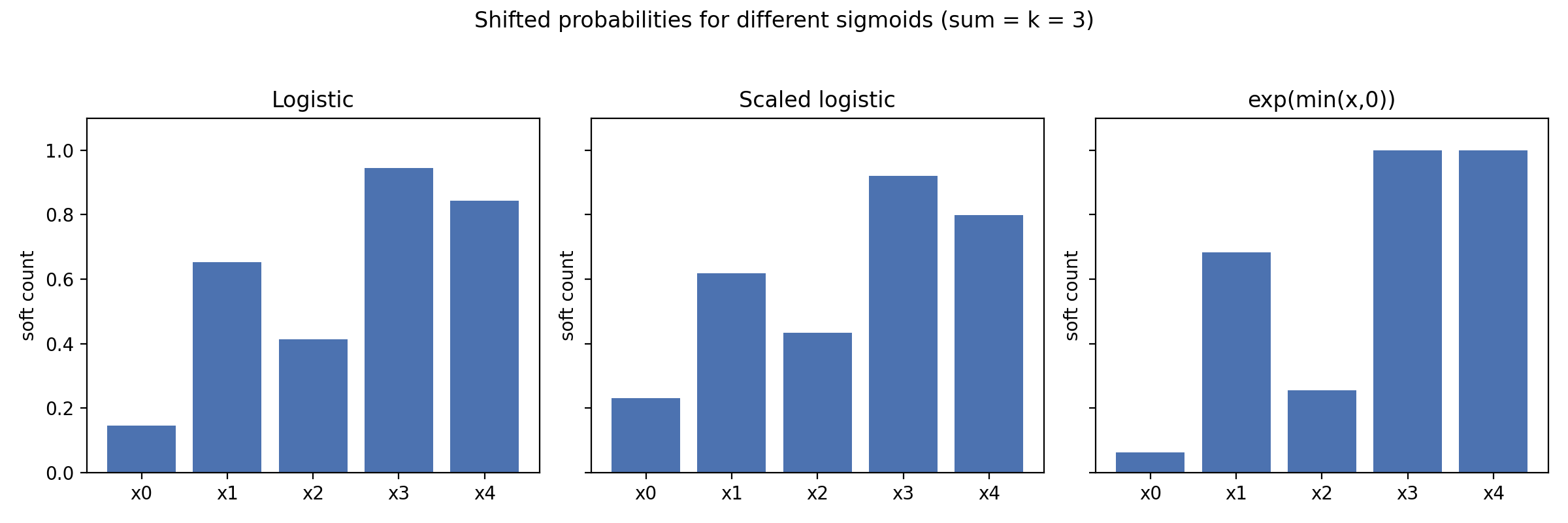
Different squashing functions bias the mass toward harder or softer selections. Using the same logits as above and solving for \(t\) in each case produces noticeably different allocations:
| \(\sigma(x)\) | Soft counts after shifting | Notes |
|---|---|---|
| Logistic \(1/(1+e^{-x})\) | [0.15, 0.65, 0.41, 0.94, 0.84] | Balanced; smoothly differentiable everywhere. |
| Scaled logistic \(1/\sqrt{1+e^{-x}}\) | [0.09, 0.67, 0.34, 0.98, 0.91] | Pushes large logits closer to 1, encouraging sparsity. |
| \(\exp(\min(x,0))\) | [0.07, 0.67, 0.27, 1.00, 1.00] | Matches softmax at \(k=1\); piecewise smooth. |
Rather than showing the code, the figure below runs that experiment directly and plots the resulting soft counts side by side.
The forward pass is only half the story. Define \(f_i(x) = \sigma(x_i + t(x))\) where \(t(x)\) is the shift that enforces the summed constraint. Start from the normalization equation \(k = \sum_i \sigma(x_i + t(x))\) and differentiate both sides with respect to \(x_j\). The left-hand side stays zero, while the right-hand side picks up both a direct term (from \(x_j\)) and an indirect term (because \(t\) itself depends on \(x_j\)):
\[0 = \sum_i \sigma'(x_i + t)\left(\delta_{ij} + \frac{\partial t}{\partial x_j}\right). \]
Pull the sum over \(\partial t/\partial x_j\) outside and solve the linear equation to get one more intermediate step, \(0 = \sigma'(x_j + t) + \frac{\partial t}{\partial x_j}\sum_i \sigma'(x_i + t)\), which rearranges to
\[\frac{\partial t}{\partial x_j} = - \frac{\sigma'(x_j + t)}{\sum_i \sigma'(x_i + t)}.\]
Plugging that back into \(\partial f_i / \partial x_j = \sigma'(x_i + t)(\delta_{ij} + \partial t / \partial x_j)\) splits the Jacobian into two recognizable parts. The diagonal contribution is just \(\sigma'(x_i + t)\) itself, while the shared \(\partial t / \partial x_j\) term turns into a rank-one matrix with entries \(-\sigma'(x_i + t)\sigma'(x_j + t)/\sum_{\ell} \sigma'(x_\ell + t)\). Writing \(v = \sigma'(x + t)\) and \(\Vert v \Vert_1 = \sum_i v_i\) we arrive at the compact expression \(J = \operatorname{diag}(v) - vv^\top / \Vert v \Vert_1\). Backpropagation never needs the dense Jacobian, only the vector–Jacobian product, which reduces to \(u \circ v - \langle u, v \rangle v / \Vert v \Vert_1\) and is both numerically stable and easy to implement.
Below is the complete implementation I shared in the answer, lightly cleaned up for readability.
It relies on functorch to evaluate \(\sigma'\) across a batch, but you can drop in your own derivative if you prefer a different \(\sigma\).
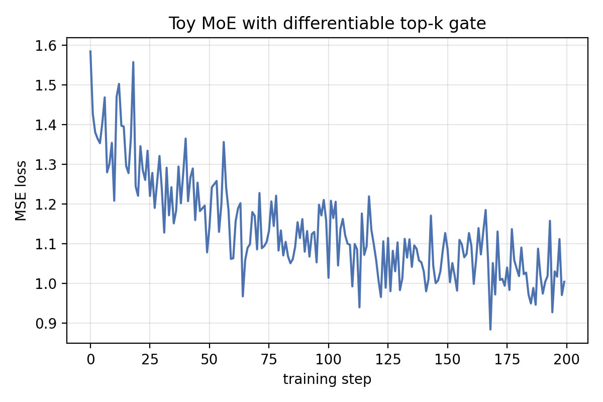
To show the operator in context, here is a tiny mixture-of-experts gate. Each expert is a linear layer; the gate scores the input, applies the differentiable top-\(k\), and forms a weighted sum. The example trains on random targets just to demonstrate that gradients flow end to end without special tricks.
class SoftMoE(torch.nn.Module):
    def __init__(self, in_dim, experts, k):
        super().__init__()
        self.scorer = torch.nn.Linear(in_dim, experts)
        self.experts = torch.nn.ModuleList(
            [torch.nn.Linear(in_dim, in_dim) for _ in range(experts)]
        )
        self.k = k

    def forward(self, x):
        scores = self.scorer(x)
        probs = TopK.apply(scores, self.k)
        expert_outs = torch.stack([layer(x) for layer in self.experts], dim=1)
        return (probs.unsqueeze(-1) * expert_outs).sum(dim=1)

model = SoftMoE(in_dim=32, experts=8, k=3)
opt = torch.optim.Adam(model.parameters(), lr=1e-3)
for step in range(200):
    x = torch.randn(16, 32)
    target = torch.randn(16, 32)
    opt.zero_grad()
    loss = torch.nn.functional.mse_loss(model(x), target)
    loss.backward()
    opt.step()
    if step % 50 == 0:
        print(step, loss.item())
Watching the printed losses drop (and optionally inspecting the gate probabilities) reassures you that the gradients remain well-behaved even though the layer enforces an exact sum-to-\(k\) constraint.
Here is a single 200-step run of that toy MoE, showing the mean-squared error steadily decreasing:
Sometimes you really do want a binary gate at inference time. The usual recipe—mirroring PyTorch’s gumbel_softmax straight-through estimator—is to keep the differentiable probabilities for gradient computation while swapping in a discrete mask on the forward path.
With the differentiable top-k this looks like:
scores = self.scorer(x)
probs_soft = TopK.apply(scores, self.k)
_, idx = torch.topk(probs_soft, self.k, dim=-1)
mask = torch.zeros_like(probs_soft).scatter_(-1, idx, 1.0)
probs_hard = mask - probs_soft.detach() + probs_soft
expert_outs = torch.stack([...], dim=1)
output = (probs_hard.unsqueeze(-1) * expert_outs).sum(dim=1)
During backprop the gradient flows through probs_soft exactly as before (because the hard mask’s contribution is detached), yet the forward signal sees a true top-k selection.
As always with straight-through estimators you trade unbiasedness for useful training dynamics, but this pattern works well when you only need hard routing at evaluation time.
torch.autograd.Function
The custom TopK layer subclasses torch.autograd.Function, so the contract is explicit: forward receives regular tensors and can write whatever auxilliary values it needs to ctx, while backward only gets the upstream gradient and those saved tensors.
Here the forward pass performs the binary search and returns the soft top-k probabilities, but it also caches both the original logits and the solved shifts \(t\).
The backward pass never recomputes \(t\); it simply rebuilds \(v = \sigma'(x + t)\), forms the vector–Jacobian product, and multiplies by the incoming gradient.
Because nothing else is saved, reverse-mode memory use stays linear in batch size.
A subtle point is that the second return value of forward (the integer k) is treated as non-differentiable, so backward returns None for that slot.
PyTorch will propagate zeros for you, but being explicit keeps the API tidy.
If you later wrap this function inside an nn.Module, the module’s forward can call TopK.apply directly and autograd will stitch the graph together just like any built-in op.
import torch
from functorch import vmap, grad
from torch.autograd import Function

sigmoid = torch.sigmoid
sigmoid_grad = vmap(vmap(grad(sigmoid)))

class TopK(Function):
    @staticmethod
    def forward(ctx, xs, k):
        ts, ps = _find_ts(xs, k)
        ctx.save_for_backward(xs, ts)
        return ps

    @staticmethod
    def backward(ctx, grad_output):
        xs, ts = ctx.saved_tensors
        v = sigmoid_grad(xs + ts)
        s = v.sum(dim=1, keepdims=True)
        uv = grad_output * v
        correction = -uv.sum(dim=1, keepdims=True) * v / s
        return uv + correction, None

@torch.no_grad()
def _find_ts(xs, k):
    b, n = xs.shape
    assert 0 < k < n
    lo = -xs.max(dim=1, keepdims=True).values - 10
    hi = -xs.min(dim=1, keepdims=True).values + 10
    for _ in range(64):
        mid = (hi + lo) / 2
        mask = sigmoid(xs + mid).sum(dim=1) < k
        lo[mask] = mid[mask]
        hi[~mask] = mid[~mask]
    ts = (lo + hi) / 2
    return ts, sigmoid(xs + ts)

TopK.apply(torch.randn(2, 3), 2)
The gist linked here contains a gradcheck harness for additional peace of mind.
Drop the layer in front of any discrete sampler, tune \(\sigma\) to control how hard you push values toward \{0,1\}, and you suddenly have a differentiable top-
k that plays nicely with backprop.
There are, of course, fancier continuous relaxations (Gumbel-topk, Sinkhorn layers, sparsemax variants), but I still like the simplicity here: one scalar constraint, one binary search, and gradients you can write down on a napkin. Sometimes that is all you need.